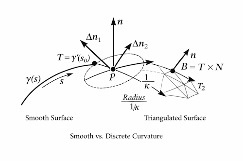
Curvature originates in the analysis of smooth curves.

\[ \gamma:I\subset\mathbb{R}\rightarrow\operatorname{R}^\mathbb{3} \]

Consider a curve parameterized by arc length s.

The unit tangent vector is defined:

\[ T\left(s\right)=\gamma^\prime\left(s\right) \]

and the curvature corresponds to the magnitude of the derivative of this tangent vector:

\[ \kappa\left(s\right)=\left\|T'\left(s\right)\right\| \]

The principal normal is defined as:

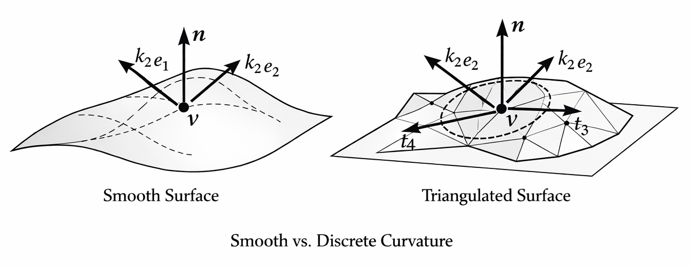
\[ N\left(s\right)=\frac{T'\left(s\right)}{\left\|T'\left(s\right)\right\|} \]

Curvature quantifies the rate at which the tangent direction changes (see Figure 1). For example, straight lines have zero curvature \(\kappa=0\), while circles of radius r exhibit constant curvature \(\kappa=1/r\).

Let \(S\) denote a smooth surface embedded in \(\mathbb{R}^3\), with a point \(p \in S\). Infinitely many smooth curves can pass through \(p\), each possessing individual curvature; however, only the component aligned with the surface normal encapsulates the surface’s curvature.

Normal curvature

Given a unit tangent direction at \(p\), and a corresponding curve \(\gamma\) on the surface such that \(\gamma\left(p\right)=0\) and \(\gamma’0=v\), the normal curvature in direction is:

\[ \kappa_n\left(v\right)=\left\langle\gamma^{\prime\prime}\left(0\right),n\left(p\right)\right\rangle \]

where \(n\left(p\right)\) is the unit normal of the surface at \(p\).

Among all possible directions:

• the maximal normal curvature is the first principal curvature \(k_1\)
• the minimal normal curvature is the second principal curvature \(k_2\)

These extremal values occur in mutually orthogonal principal directions, forming the principal curvature frame (see Figure 2).

Mean and Gaussian curvature

Two scalar invariants summarize the local geometry:

\[ H=\frac{k_1+k_2}{2},    K=k_1k_2. \]

These invariants assist in classifying local surface shape.

Shape type	Gaussian curvature (K)	Description
Elliptic	\(K>0\)	Dome-like, both curvatures same sign
Hyperbolic	\(K<0\)	Saddle-like
Parabolic	\(K=0\)	Cylindrical
Planar	\(k_1=k_2=0\)	Flat

The most sophisticated formulation of curvature arises through the shape operator (Weingarten map).

Definition

Let \(n:S\rightarrow\mathbb{S}^\mathbb{2}\) be the unit normal field. The shape operator is:

\[S_p:T_pS\rightarrow T_pS,    S_p\left(v\right)=-D_vn,\]

the negative directional derivative of the normal field.

Significance

The eigenvalues of \(S_p\) are the principal curvatures \(\operatorname{k}_1,\ \operatorname{k}_2\), and the eigenvectors identify their directions.

The second fundamental form is

\[\mathrm{II}\left(u,v\right)=\left\langle S\left(u\right),v\right\rangle.\]

Thus:

Curvature is fundamentally encoded in variations of the normal field.

The shape operator succinctly captures these variations (see Figure 3), forming the basis of modern discrete curvature estimators.

Triangle meshes are inherently piecewise linear structures. They lack:

• smooth derivatives,
• continuous tangent planes,
• consistent normals across edges,
• intrinsic curvature.

Despite these limitations, there is a persistent need to approximate smooth curvature using discrete representations.

Key Challenges

• Normal discontinuity: Normals exhibit abrupt changes along edges.
• Neighborhood ambiguity: “Locality” is ill-defined on irregular meshes.
• Noise sensitivity: Curvature magnifies noise artifacts.
• Sampling irregularity: Variability in triangle size and shape affects accuracy.
• Absence of smoothness: The shape operator requires derivatives unavailable on piecewise linear surfaces.

Discontinuous normals at mesh edges (see Figure 4) render accurate curvature estimation particularly challenging.

Several methodologies exist for approximating curvature on triangle meshes:

1. Angle deficit (Gaussian curvature)

\[ \left(v\right)\approx\frac{2\pi-\sum\theta_i}{A_v} \]

Provides Gaussian curvature exclusively at vertices, with limited scope.

2. Cotangent Laplacian (mean curvature normal)

\[ Hn\approx\frac{1}{2A_v}\sum_{\left(i,j\right)}\left(\cot{\alpha_{ij}}+\cot{\beta_{ij}}\right)\left(x_i-x_j\right) \]

A widely adopted discrete differential operator.

3. Quadratic fitting

Employs local polynomial surface fitting and analytical extraction of curvature.

4. PCA-based methods

Estimates curvature directions via covariance analysis of points or normals.

5. Normal cycle curvature tensor

Integrates normal variation throughout the neighborhood, closely approximating the shape operator.

Among these, the normal cycle approach aligns most closely with the principles of smooth differential geometry and forms the foundation of the forthcoming curvature module.

The robustness and theoretical grounding of these approaches vary considerably (see Figure 5).

In the context of smooth surfaces, curvature is encapsulated within the shape operator,

\[S\ =\ -D\ n,\]

representing the negative derivative of the normal field. On triangle meshes, the normal field is piecewise constant with its derivative distributed along edges. Approximating the smooth operator entails integrating normal variation over localized neighborhoods to construct a discrete curvature tensor.

Multiple formulations exist within the literature. Below, we present the most prevalent and theoretically robust variants.

1. Normal Variation Across Edges

For a vertex \(v\), let incident edges \(e_i\) be shared by faces with normals \(n_i^+\) and \(n_i^-\). The normal jump across edge \(e_i\) is:

\[\Delta n_i=n_i^+-n_i^-.\]

Let \(t_i\) denote the unit tangent direction along edge \(e_i\) and \(l_i\) the edge length.

The underlying principle is:

Normal variation across an edge approximates the directional derivative of the normal field.

Therefore, a discrete approximation to the shape operator's contribution from edge \(e_i\) is:

\[S_i\approx\frac{\Delta n_i\otimes t_i}{\operatorname{l}_i}\]

where \(\otimes\) represents the outer product.

Each edge provides a directional term capturing normal variation (see Figure 6).

2. Area‑Weighted Curvature Tensor

To aggregate contributions from all edges surrounding vertex \(v\), weights based on the dual area \(A_v\) (often the mixed Voronoi area) are applied:

\[A_v=\frac{1}{8}\sum_{i,j}(\cot\alpha_{ij}+\cot\beta_{ij})\|x_i-x_j\|^2.\]

The discrete curvature tensor thus becomes:

\[S_v=\frac{1}{2A_v}\sum_{e_i\in\mathrm{1-ring} \left(v\right)}\ell_i,\left(\Delta n_i\otimes t_i\right)\]

This is the discrete analogue of the smooth shape operator.

Interpretation

• \(t_i\) delineates movement direction along the surface.
• \(\Delta n_i\) describes normal rotation.

The tensor \(S_v\) characterizes how normal rotation depends on directionality.

3. Symmetrized Curvature Tensor

To retain symmetry—an intrinsic property of the continuous shape operator—the discrete tensor is often symmetrized:

\[\widetilde{S_v}=\frac{1}{2}\left(S_v+S_v^\top\right)\]

This adjustment enhances numerical stability and guarantees real eigenvalues.

4. Principal Curvatures and Directions

Eigenanalysis of \(\widetilde{S_v}\) yields the discrete principal curvatures and directions:

\[\widetilde{S_v} e_1 = k_1 e_1, \quad \widetilde{S_v} e_2 = k_2 e_2.\]

Scalar curvatures are easily extracted:

\[ H = \frac{k_1 + k_2}{2}, \quad K = k_1 k_2. \]

Visualizations may depict this tensor as an ellipse in the tangent plane (see Figure 7).

5. Tensor from Normal Covariance (Normal Cycles)

An alternative formulation uses the covariance of normals in the 1 ring:

\[C_v=\sum_{f\in\mathrm{1-ring}\left(v\right)} A_f,\left(n_f-\bar{n}\right)\otimes\left(n_f-\bar{n}\right),\]

where

\[\bar{n}=\frac{1}{\sum A_f}\sum{A_fn_f}.\]

This tensor records normal variability around the vertex. Projection onto the tangent plane yields a curvature tensor:

\[S_v=P_v,C_v,P_v\]

where

\[P_v=I-n_v\otimes n_v\]

denotes tangent-plane projection.

This robust formulation is extensively utilized in geometry processing and accurately reflects curvature information (see Figure 8).

6. Tensor from Edge-Based Normal Cycles

A refined approach integrates normal variation along edges:

\[C_v=\sum_{e_i}\theta_i \ell_i \left(b_i\otimes b_i\right),\]

where:

• \(\theta_i\) is the dihedral angle at edge \(e_i\),
• \(b_i\) is the unit binormal direction,
• \(\ell_i\) denotes edge length.

Then:

\[S_v=\frac{1}{A_v}P_vC_vP_v.\]

This is the discrete counterpart to smooth integration of the second fundamental form over neighborhoods, reliably mirroring smooth curvature behavior (see Figure 9).

Curvature constitutes a profound geometric concept grounded in differential geometry. A comprehensive understanding of curvature on smooth surfaces—including normal curvature, principal curvatures, and the shape operator—provides the necessary conceptual foundations for developing robust discrete curvature estimators for triangle meshes.

Forthcoming Developments

The next article will address the implementation of a practical curvature module designed to:

• construct discrete curvature tensors,
• extract principal curvatures and directions,
• manage noise and sampling irregularities,
• integrate seamlessly into finite element and segmentation pipelines.