
Curvature Estimation on Triangle Meshes: From Theory to Implementation
Introduction
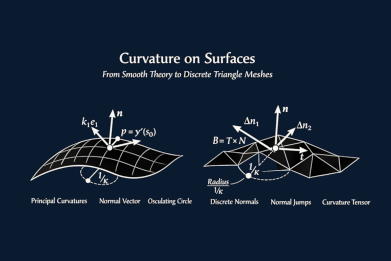
The preceding article introduced curvature from the perspective of smooth differential geometry, describing how surfaces bend, the manner in which normal fields encode curvature, and how the shape operator encapsulates this bending in a linear format. This second installment applies those theoretical concepts to develop a practical pipeline for curvature estimation on triangular meshes. The implementation provided here corresponds exactly to the GitHub module referenced earlier—an approach that is:
- mathematically rigorous
- computationally efficient
- straightforward to implement
- robust enough for real world mesh applications
It facilitates computation of:
- Gaussian curvature, via the angle defect method
- Mean curvature, using the cotangent Laplace-Beltrami operator
- Principal curvatures and directions via a least squares fit of the discrete shape operator
Collectively, these measures supply a comprehensive characterization of curvature at each mesh vertex.
Preprocessing: Preparing the Mesh for Curvature Computation
Curvature is inherently a local differential quantity; hence, reliable geometric information must be available prior to computation. The presented implementation ensures this by performing three preprocessing steps:
Face properties
Each face records:
- area
- normal
- adjacency information
These properties are computed once and reused throughout the curvature estimation pipeline.
Vertex normals
Vertex normals are calculated as angle-weighted averages of incident face normals, yielding smooth and stable normals suitable for projection and least-squares fitting.
Voronoi (mixed) areas
Each vertex maintains a mixed area as a discretized representation of the local surface area surrounding the vertex. This mixed area normalizes curvature values, ensuring scale-independent results. The high-level function `compute_vertex_curvatures` automatically completes these preprocessing steps before curvature computations commence.
Gaussian Curvature: Angle Defect Over Mixed Area
Gaussian curvature quantifies surface bending in two orthogonal directions simultaneously. In smooth geometry, it equals the product of principal curvatures; on a mesh, it is approximated through the angle defect method.
Angle Defect
At each vertex, the sum of angles from all incident triangles gives:
\[\sum\theta_i\]For interior vertices:
\[K=\frac{2\pi-\sum\theta_i}{A_{\mathrm{mixed}}}\]For boundary vertices:
\[K=\frac{\pi-\sum\theta_i}{A_{\mathrm{mixed}}}\]This technique is implemented directly within the codebase.
double angle_defect = 2.0 * PI<double> - v->angle_sum;
if (v->is_boundary) {
    angle_defect = PI<double> - v->angle_sum;
}
v->curvature_info.gaussCurvature = angle_defect / area_mixed;
Interpreting Gaussian Curvature
Curvature sign is classified as follows:
- positive: dome-like (elliptic)
- negative: saddle-like (hyperbolic)
- near zero: cylindrical or flat (parabolic)
Such classification is beneficial for tasks including segmentation and feature detection.
Mean Curvature: Cotangent Laplace-Beltrami Operator
Mean curvature assesses average surface bending. Conceptually, in the smooth domain:
\[H=\frac{k_1+k_2}{2}\]On a mesh, we compute it using the cotangent Laplacian, a standard tool in discrete differential geometry.
Cotangent Weights
For each edge \left(v_i,v_j\right), the cotangent weights are computed as follows:
\[w_{ij}=\frac{\cot{\alpha}+\cot{\beta}}{2}\]Where \alpha and \beta are the angles opposite the edge in adjacent triangles are utilized. The function `computeCotangentWeight` implements this precisely.
Discrete Laplacian
The Laplacian at vertex v is formulated as:
\[\Delta p=\sum_{j}{w_{ij}\left(p_j-p_i\right)}\]In code:
laplace += cot_weight * (neighbor->position - v->position);
Mean Curvature Value
Calculation proceeds as:
\[H=\frac{1}{2A_{\mathrm{mixed}}}\left\langle\Delta p,n\right\rangle\]This matches the continuous formulation, wherein the Laplacian of the embedding yields twice the mean curvature normal.
Principal Curvatures and Directions: Least-Squares Shape Operator
This section constitutes the most sophisticated component of the implementation and aligns directly with the theory described previously.
Local Tangent Frame
At each vertex, an orthonormal basis is constructed:
- \(n\): vertex normal
- \(t_1, t_2\): tangent vectors spanning the tangent plane
This configuration establishes a local coordinate system facilitating linear treatment of curvature.
Normal Variation
For each neighboring vertex:
- Project the positional difference onto the tangent plane,
- Project the normal difference onto the tangent plane,
These samples describe how the normal field varies around the vertex.
Fitting the Shape Operator
Assume:
\[\Delta n \approx S \Delta p\]where \(S\) denotes the \(2 \times 2\) symmetric shape operator. A least-squares solution determines the operator entries, offering a stable and widely adopted approach.
Eigen-Decomposition
Once \(S\) is determined:
- Eigenvalues represent principal curvatures,
- Eigenvectors indicate principal directions,
Mapping eigenvectors back into 3D space completes the curvature characterization at every vertex.
Numerical Stability and Practical Considerations
The implementation incorporates several safeguards:
- fallback mechanisms for insufficient neighbors,
- Gaussian elimination with pivoting,
- normalization of eigenvectors,
- curvature sign classification,
- boundary vertex handling.
These refinements ensure reliability for real mesh data, not just idealized models.
Consolidating the Pipeline
The function `computeMeshCurvatures` iterates over all vertices, calculating:
- Gaussian curvature,
- mean curvature,
- principal curvatures,
- principal directions.
The output forms a rich geometric dataset applicable to:
- segmentation,
- feature line extraction,
- smoothing,
- remeshing,
- shape analysis,
- visualization.
This pipeline offers a complete, theoretically-grounded solution with a clean implementation.
Conclusion and Future Extensions
The curvature module described herein is designed to be simple, robust, and educational. It provides an effective solution consistent with theoretical principles, absent excessive complexity. Potential future articles may address advanced topics such as:
- normal cycles,
- geodesic neighborhoods,
- curvature tensor smoothing,
- quadric fitting,
- multi-scale curvature,
- curvature flow.
These subjects will naturally extend the foundation established by the present work.

Source Code
To review the full implementation—the exact curvature module discussed—visit GitHub:
https://github.com/cosfer65/themeshprojectA compact and reliable curvature pipeline for study, adaptation, or direct integration into mesh processing tools.